
I remember the first time I trained a neural network that actually worked. Not a toy example from a tutorial, but a model that solved a real problem a client had been struggling with for months. The moment the validation loss curve flattened into a smooth descent and the test accuracy crossed 94%, I realised something profound: deep learning is not just another tool in the software engineer's toolbox. It represents a fundamentally different paradigm of programming, one where we stop writing explicit rules and start teaching machines to discover patterns from data. That shift, quiet as it was, has reshaped entire industries.
Over the past decade, deep learning has evolved from an academic curiosity into the engine behind search engines, voice assistants, medical diagnostics, autonomous vehicles, and the large language models powering tools like ChatGPT and Claude. Despite the hype, the core principles remain surprisingly stable. This article is my attempt to explain those principles the way I wish someone had explained them to me when I started: from first principles, with engineering intuition, practical code, and honest discussions of where things break.
We will cover a lot of ground. From the mathematics of a single artificial neuron to the architecture of modern transformers, from writing your first training loop in PyTorch to understanding why mixed-precision training matters in production. Every section is written to stand on its own, but together they form a complete map of the field as it exists in 2026. If you are a developer, a student, a researcher, or a business leader trying to understand what deep learning can and cannot do, this resource is built for you.
What Is Deep Learning? A Working Definition
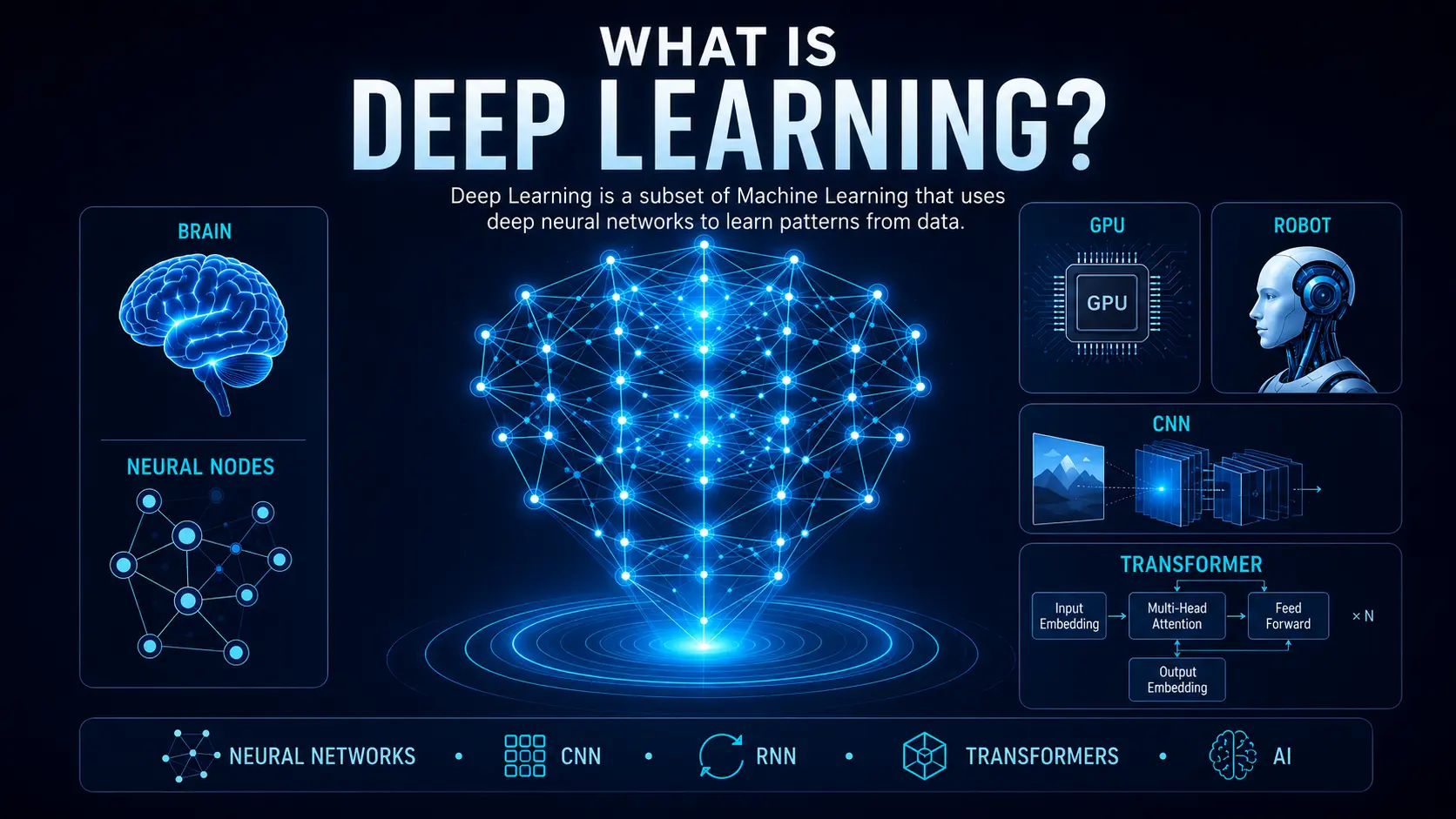
Deep learning is a subfield of machine learning that uses artificial neural networks with multiple layers (hence "deep") to learn hierarchical representations of data. Instead of relying on hand-crafted features, a deep learning model ingests raw data, passes it through successive layers of computation, and automatically discovers the features that matter most for the task at hand. This process, called representation learning, is what separates deep learning from classical machine learning approaches.
Consider an image classifier. In traditional machine learning, an engineer might spend weeks designing edge detectors, colour histograms, and texture descriptors before training a model. With deep learning, you feed raw pixel values into a convolutional neural network. The first layer might learn to detect edges, the second layer combines edges into shapes, the third recognises parts of objects, and the final layers assemble these into whole-object representations. The model builds its own feature hierarchy, and it usually discovers better features than humans can design by hand.
This does not mean deep learning is magic. It requires vast amounts of labelled data, significant computational resources, and careful engineering to work reliably. But when these conditions are met, deep learning consistently outperforms every other approach we have for tasks like image recognition, speech synthesis, machine translation, and protein structure prediction. The fundamental insight, that compositionality and depth enable increasingly abstract representations, has proven remarkably robust across domains.
The Relationship Between AI, Machine Learning, and Deep Learning
These terms are often used interchangeably in marketing material, but they describe nested concepts with important distinctions. Understanding the hierarchy helps when scoping projects and communicating with stakeholders.
| Term | Scope | Examples |
|---|---|---|
| Artificial Intelligence (AI) | The broadest field. Any system that exhibits intelligent behaviour. | Rule-based chess engines, expert systems, pathfinding algorithms, AI assistants |
| Machine Learning (ML) | A subset of AI. Systems that learn patterns from data without being explicitly programmed for every scenario. | Linear regression, decision trees, SVMs, random forests, gradient boosting |
| Deep Learning (DL) | A subset of ML. Uses multi-layered neural networks to learn hierarchical representations. | CNNs for vision, transformers for language, GANs for image generation, diffusion models |
The key distinction is that deep learning models learn features automatically, whereas classical ML typically requires manual feature engineering. For a deeper exploration of AI categories beyond just narrow systems, see the guide on Narrow AI vs AGI vs Superintelligence and the overview of types of artificial intelligence.
A Brief History of Deep Learning
The intellectual roots of deep learning stretch back further than most people realise. In 1943, Warren McCulloch and Walter Pitts published a mathematical model of a biological neuron, proposing that binary threshold units could compute logical functions. Frank Rosenblatt's perceptron, unveiled in 1958, was the first hardware implementation of a trainable neural network. It could learn to classify simple patterns, and the press of the time speculated wildly about its potential. Then came the first AI winter.
Marvin Minsky and Seymour Papert's 1969 book Perceptrons demonstrated that single-layer perceptrons could not solve the XOR problem, a simple non-linearly separable function. Funding dried up, and neural network research languished for over a decade. The revival began in the 1980s with the invention of backpropagation, popularised by Rumelhart, Hinton, and Williams in 1986, which provided an efficient way to train multi-layer networks. Yet even then, vanishing gradients and limited compute kept networks shallow.
The modern era began in earnest around 2012. Alex Krizhevsky, Ilya Sutskever, and Geoffrey Hinton entered the ImageNet competition with a deep convolutional neural network trained on GPUs. Their model, AlexNet, achieved a top-5 error rate of 15.3%, nearly halving the previous best. That moment crystallised what many researchers had suspected: with enough data, enough compute, and the right architectural innovations, deep neural networks could achieve superhuman performance on narrowly defined tasks. The GPU era had begun, and the rest, as they say, is history written in Tensor Cores and attention mechanisms.
How Deep Learning Actually Works: From Neurons to Training Loops
The Artificial Neuron
Everything starts with a single artificial neuron. It takes a vector of inputs \(\mathbf{x} = [x_1, x_2, \dots, x_n]\), multiplies each by a corresponding weight \(w_i\), sums the results, adds a bias term \(b\), and passes the total through an activation function \(f\). Mathematically:
\[ y = f\left(\sum_{i=1}^{n} w_i x_i + b\right) = f(\mathbf{w} \cdot \mathbf{x} + b) \]The weights determine how much influence each input has. The bias shifts the decision boundary, allowing the neuron to fire even when all inputs are zero. The activation function introduces non-linearity. Without it, stacking multiple layers would collapse into a single linear transformation, no matter how many layers you added. Common activation functions include ReLU, sigmoid, tanh, GELU, and Swish. We will examine each in the activation functions section below.
The Perceptron and Its Limitations
The original perceptron used a step function as its activation: output 1 if the weighted sum exceeded a threshold, 0 otherwise. This made it a linear binary classifier. It worked well for linearly separable problems, but as Minsky and Papert proved, a single perceptron cannot solve XOR. The solution was to stack perceptrons into layers and use differentiable activation functions, enabling gradient-based training through backpropagation. This architectural leap from single perceptron to multi-layer perceptron is the conceptual foundation of all modern deep learning.
Neural Network Architecture
A feedforward neural network, also called a multi-layer perceptron (MLP) or artificial neural network (ANN), consists of an input layer, one or more hidden layers, and an output layer. Each layer is a collection of neurons whose outputs become the inputs to the next layer. Information flows strictly forward during inference. The number of neurons in each hidden layer and the total number of hidden layers define the network's width and depth respectively. Wider networks can memorise more patterns; deeper networks can learn more abstract, compositional features. The trade-off is that deeper networks are harder to train due to vanishing gradients, a problem addressed by architectural innovations like residual connections and normalisation layers.
Forward Propagation
Forward propagation is the process of computing the network's output for a given input. Starting from the input layer, each layer's output is computed as the activation of the weighted sum of the previous layer's outputs plus biases. This cascades through the network until the final layer produces predictions. For a layer with weight matrix \(\mathbf{W}\), bias vector \(\mathbf{b}\), and input \(\mathbf{x}\), the forward pass computes \(\mathbf{a} = f(\mathbf{W}\mathbf{x} + \mathbf{b})\). During training, these intermediate activations are stored because backpropagation needs them to compute gradients. During inference, only the final output matters, which opens opportunities for optimisation like layer fusion and activation caching.
Loss Functions
A loss function quantifies how wrong the model's predictions are. During training, we minimise this value. Different tasks demand different loss functions. For binary classification, binary cross-entropy compares predicted probabilities against true labels. For multi-class classification with mutually exclusive classes, categorical cross-entropy with a softmax output layer is standard. For regression, mean squared error (MSE) penalises large errors quadratically, while mean absolute error (MAE) is more robust to outliers. For segmentation tasks, Dice loss or focal loss often works better. Choosing the right loss function is one of the most consequential design decisions in any deep learning project.
\[ \mathcal{L}_{\text{CE}} = -\sum_{c=1}^{C} y_c \log(\hat{y}_c) \]Here, \(y_c\) is 1 if \(c\) is the correct class and 0 otherwise, and \(\hat{y}_c\) is the predicted probability for class \(c\). The softmax function, \(\hat{y}_c = \frac{e^{z_c}}{\sum_{j} e^{z_j}}\), ensures outputs sum to 1 and can be interpreted as probabilities.
| Loss Function | Typical Use Case | Characteristics |
|---|---|---|
| Binary Cross-Entropy | Binary classification | Outputs interpreted as probabilities; numerically unstable without clipping |
| Categorical Cross-Entropy | Multi-class classification | Used with softmax; assumes mutually exclusive classes |
| Mean Squared Error | Regression | Sensitive to outliers; differentiable everywhere |
| Mean Absolute Error | Regression (robust) | Less sensitive to outliers; non-differentiable at zero |
| Huber Loss | Regression | Combines MSE and MAE; smooth near zero |
| Focal Loss | Imbalanced classification | Down-weights well-classified examples; useful for object detection |
| Dice Loss | Image segmentation | Optimises overlap directly; handles class imbalance well |
| CTC Loss | Sequence recognition | Aligns unsegmented sequences; used in speech recognition |
Gradient Descent and the Learning Rate
Gradient descent is the iterative optimisation algorithm that adjusts the network's weights to minimise the loss. At each step, we compute the gradient of the loss with respect to every parameter. The gradient points in the direction of steepest increase, so we move in the opposite direction. The size of that step is the learning rate. Too large, and training diverges or oscillates. Too small, and training crawls or gets stuck in local minima. Finding the right learning rate is more art than science, though schedulers like cosine annealing, warm-up, and cyclical learning rates have made it more systematic.
\[ \theta_{t+1} = \theta_t - \eta \nabla_\theta \mathcal{L}(\theta_t) \]Here, \(\theta_t\) represents all model parameters at step \(t\), \(\eta\) is the learning rate, and \(\nabla_\theta \mathcal{L}\) is the gradient of the loss. In practice, pure gradient descent is almost never used. Mini-batch stochastic gradient descent and adaptive optimisers dominate.
Optimisers
The choice of optimiser affects convergence speed, final performance, and training stability. SGD with momentum adds a velocity term that smooths the update direction and helps escape shallow local minima. Adam combines momentum with adaptive per-parameter learning rates based on first and second moments of gradients, making it a robust default for many problems. AdamW decouples weight decay from the adaptive learning rate, which often yields better generalisation. RMSProp remains popular for recurrent networks. Recently, Lion (discovered through evolutionary search) has shown promise, and Shampoo brings second-order information at scale.
| Optimiser | Key Mechanism | Best For | Weakness |
|---|---|---|---|
| SGD + Momentum | Velocity-accelerated gradient descent | Image classification with CNNs | Requires careful LR tuning |
| Adam | Adaptive moments (1st & 2nd) | General purpose; NLP; GANs | Can generalise worse than SGD |
| AdamW | Decoupled weight decay | Transformers; fine-tuning | Slightly more hyperparameters |
| RMSProp | Adaptive learning rates via moving average of squared gradients | RNNs; LSTMs | No momentum term by default |
| Lion | Sign-based updates; evolution-discovered | Large language models | Newer; less community experience |
| LAMB / LARS | Layer-wise adaptive rates | Large-batch training | Complexity overhead |
Backpropagation
Backpropagation is the algorithm that makes training deep networks computationally feasible. It applies the chain rule of calculus to compute the gradient of the loss with respect to every parameter in the network, working backwards from the output layer to the input. For each layer, it multiplies the upstream gradient by the local gradient of that layer's operation. This avoids the exponential blow-up that would occur if we tried to compute gradients by perturbing each parameter individually. The computational graph framework used by PyTorch (autograd) and TensorFlow (GradientTape) automates this process, allowing engineers to define arbitrary differentiable operations and get gradients for free.
Activation Functions in Detail
The choice of activation function profoundly affects training dynamics. ReLU (Rectified Linear Unit), \(f(x) = \max(0, x)\), became dominant because it avoids the vanishing gradient problem that plagued sigmoid and tanh in deep networks. However, ReLU neurons can "die" if they consistently receive negative inputs, outputting zero forever. Leaky ReLU and Parametric ReLU address this with a small negative slope. GELU (Gaussian Error Linear Unit) has become the standard in transformer architectures because its smooth, probabilistic gating works well with layer normalisation. Swish, discovered through neural architecture search, sometimes outperforms ReLU in very deep networks.
| Function | Formula | Range | Key Property |
|---|---|---|---|
| Sigmoid | \(\sigma(x) = \frac{1}{1+e^{-x}}\) | (0, 1) | Smooth; saturates at extremes; vanishing gradients |
| Tanh | \(\tanh(x) = \frac{e^x - e^{-x}}{e^x + e^{-x}}\) | (-1, 1) | Zero-centred; still saturates |
| ReLU | \(f(x) = \max(0, x)\) | [0, ∞) | Non-saturating for x>0; dying neuron problem |
| Leaky ReLU | \(f(x) = \max(0.01x, x)\) | (-∞, ∞) | Prevents dead neurons; fixed negative slope |
| GELU | \(x \cdot \Phi(x)\) | (-∞, ∞) | Smooth; probabilistic gating; standard in transformers |
| Swish | \(x \cdot \sigma(\beta x)\) | (-∞, ∞) | Self-gated; learnable β; discovered by NAS |
| SiLU | \(x \cdot \sigma(x)\) | (-∞, ∞) | Equivalent to Swish with β=1; common in ConvNeXt |
Epochs, Iterations, and Batch Size
An epoch is one complete pass through the entire training dataset. An iteration is one gradient update step, processing a single mini-batch. The batch size is the number of samples processed before updating weights. These three quantities are related: number of iterations per epoch = total samples / batch size. Larger batch sizes provide more accurate gradient estimates but require more GPU memory and can lead to poorer generalisation (the "generalisation gap" phenomenon). Smaller batches introduce helpful noise that aids exploration. In practice, the batch size is often chosen as the largest value that fits in GPU memory, with gradient accumulation used to simulate larger effective batches when needed.
Weights and Biases
Weights are the multiplicative parameters that scale input signals. Biases are additive offsets that shift activation thresholds. Together, they define the affine transformation at each layer before the activation function. Proper initialisation of weights is critical. If weights start too large, gradients explode. If they start too small, gradients vanish, especially in deep networks with saturating activations. Xavier/Glorot initialisation scales weights based on fan-in and fan-out for tanh activations. He initialisation, designed for ReLU, scales by \(\sqrt{2 / \text{fan-in}}\) to account for the fact that ReLU zeros out half the activations in expectation. Modern frameworks handle this automatically, but understanding the rationale helps when debugging training issues.
Feature Engineering vs Representation Learning
In classical machine learning, feature engineering is the process of manually designing informative input representations. An engineer might spend weeks crafting features for a fraud detection model: transaction frequency, average transaction amount, time since last transaction, and so on. Deep learning shifts this burden to the model. The raw data goes in, and the network learns its own features through the training process. This is representation learning. It is more data-hungry and compute-intensive, but it often discovers patterns that human engineers miss. In practice, hybrid approaches work best for structured data: use domain knowledge to create a sensible input representation, then let the deep model refine it.
Training vs Inference
Training is the computationally expensive phase where the model learns from labelled data. It involves forward propagation, loss computation, backpropagation, and weight updates. GPUs, TPUs, and distributed clusters are typically required. Inference is the deployment phase where the trained model makes predictions on new data. Inference requires only forward propagation and can be heavily optimised through quantisation, pruning, kernel fusion, and specialised hardware. Understanding this dichotomy is essential for production ML engineering. A model that takes days to train on 8 GPUs might run inference on a mobile phone in under 10 milliseconds after optimisation.
Learning Paradigms: How Models Acquire Knowledge
Supervised Learning
Supervised learning is the most common paradigm in deep learning. The training data consists of input-output pairs, and the model learns a mapping from inputs to outputs by minimising a loss function that compares predictions to ground-truth labels. Image classification, speech recognition, sentiment analysis, and most structured prediction tasks fall under this category. The primary limitation is the need for large quantities of accurately labelled data, which is expensive and time-consuming to produce.
Unsupervised Learning
Unsupervised learning works with unlabelled data, seeking to uncover hidden structure. Clustering, dimensionality reduction, anomaly detection, and density estimation are classical examples. In deep learning, autoencoders and self-organising maps are traditional unsupervised architectures. More recently, generative models like GANs and diffusion models blur the line between unsupervised and self-supervised learning by learning data distributions without explicit labels.
Self-Supervised Learning
Self-supervised learning has become one of the most exciting frontiers. The idea is deceptively simple: create a "pretext" task from the data itself that generates labels for free. For text, this might involve predicting masked words (as in BERT) or the next token (as in GPT). For images, contrastive methods like SimCLR and MoCo learn representations by pulling augmented views of the same image together and pushing different images apart. Self-supervised pre-training on enormous unlabelled corpora, followed by supervised fine-tuning on smaller labelled datasets, is the dominant paradigm behind modern foundation models.
Transfer Learning and Fine-Tuning
Transfer learning takes a model trained on one task and repurposes it for a related task. In computer vision, it is standard practice to start from a model pre-trained on ImageNet and fine-tune it on a smaller domain-specific dataset. This works because the early layers of a CNN learn general visual features like edges and textures that transfer across domains. Fine-tuning involves unfreezing some or all of the pre-trained layers and continuing training on the new task, usually with a much lower learning rate. The same principle applies to large language models: pre-train on massive text corpora, then fine-tune on instruction-following data or domain-specific documents.
Foundation Models
Foundation models are large-scale models trained on broad data at immense computational cost, designed to be adapted to a wide range of downstream tasks. GPT-4, Claude, Gemini, Llama 3, and Stable Diffusion are all foundation models. They are characterised by emergent abilities that were not explicitly programmed, such as in-context learning and chain-of-thought reasoning. The Retrieval-Augmented Generation (RAG) pattern combines foundation models with external knowledge bases to ground outputs in factual information. For a practical walkthrough, the ChatGPT beginner's guide and the Claude AI master guide provide hands-on perspectives on working with these systems.
Embeddings, Latent Spaces, and Vector Representations
An embedding is a dense, low-dimensional vector representation of a discrete or high-dimensional input. Words, images, user profiles, and even entire documents can be embedded into continuous vector spaces where semantically similar items cluster together. The latent space is the abstract, lower-dimensional manifold that the model learns to represent its inputs. Operations in this space can be surprisingly meaningful: in word embedding spaces, the vector arithmetic \(\text{king} - \text{man} + \text{woman} \approx \text{queen}\) famously demonstrates how relational knowledge is encoded geometrically.
Model parameters are the learned weights and biases of the network. Hyperparameters are the settings configured before training: learning rate, batch size, number of layers, dropout rate, and so on. Model architecture refers to the structural design of the network, the types and arrangement of layers, connections, and operations. These three concepts form a hierarchy: architecture constrains what can be learned, hyperparameters control how learning proceeds, and parameters embody what has been learned.
Generalisation, Overfitting, and Regularisation
Overfitting and Underfitting
Overfitting occurs when a model memorises the training data instead of learning generalisable patterns. It performs brilliantly on training examples but poorly on unseen data. Underfitting is the opposite: the model is too simple to capture the underlying patterns, and performance is poor on both training and test sets. The goal of training is to find the sweet spot between these two failure modes, a concept formalised as the bias-variance trade-off.
Regularisation Techniques
L1 and L2 regularisation add penalty terms to the loss function based on the magnitude of the weights. L1 encourages sparsity by driving some weights to exactly zero. L2 discourages large weights, producing smoother models. Dropout, one of the most effective regularisation techniques, randomly deactivates a fraction of neurons during each training iteration, forcing the network to develop redundant representations that generalise better. At inference time, dropout is disabled, and weights are scaled appropriately.
Batch Normalisation
Batch normalisation normalises the activations of each layer to have zero mean and unit variance across the mini-batch, then applies learnable scale and shift parameters. This stabilises training, allows higher learning rates, reduces sensitivity to weight initialisation, and has a mild regularising effect due to the noise introduced by batch statistics. Layer normalisation, which normalises across features rather than batch elements, has become the standard in transformer architectures because it works consistently across batch sizes and is compatible with sequence models.
Data Augmentation and Cross-Validation
Data augmentation artificially expands the training set by applying label-preserving transformations: random crops, flips, rotations, and colour jitter for images; synonym replacement and back-translation for text; time stretching and pitch shifting for audio. It is one of the most reliable ways to improve generalisation. Cross-validation partitions the data into multiple folds, training on some and validating on others in rotation, providing a more robust estimate of model performance than a single train-test split.
Evaluation Metrics Beyond Accuracy
| Metric | Formula / Description | Best Used When |
|---|---|---|
| Accuracy | Correct predictions / Total predictions | Balanced classes; simple benchmark |
| Precision | TP / (TP + FP) | Cost of false positives is high |
| Recall (Sensitivity) | TP / (TP + FN) | Cost of false negatives is high |
| F1 Score | 2 × (Precision × Recall) / (Precision + Recall) | Imbalanced classes; need single summary |
| ROC-AUC | Area under ROC curve; TPR vs FPR | Binary classification; threshold-independent |
| PR-AUC | Area under precision-recall curve | Highly imbalanced datasets |
| Confusion Matrix | Table of TP, FP, TN, FN | Detailed error analysis |
| IoU (Jaccard) | Intersection over Union | Object detection; segmentation |
| Perplexity | Exponentiated cross-entropy | Language modelling |
| BLEU / ROUGE | N-gram overlap with reference | Machine translation; summarisation |
A common beginner mistake is optimising for accuracy when the dataset is 99% negative class. A model that predicts "negative" every time achieves 99% accuracy and is completely useless. Precision, recall, and F1 score tell a more honest story. For business stakeholders, it is often more meaningful to translate these metrics into expected cost savings, error rates per thousand transactions, or customer experience improvements.
Major Deep Learning Architectures
Artificial Neural Networks (ANN / MLP)
Purpose: General-purpose function approximation. Architecture: Fully connected layers where each neuron connects to every neuron in the adjacent layers. Advantages: Simple, well-understood, works on tabular data. Disadvantages: Ignores spatial and sequential structure; parameter count explodes with input size. Applications: Tabular data, simple regression and classification, baseline models. Limitations: Cannot efficiently process images or sequences without prohibitive parameter counts.
Convolutional Neural Networks (CNN)
Purpose: Processing grid-structured data, especially images. Architecture: Convolutional layers apply learnable filters that slide across the input, detecting local patterns. Pooling layers reduce spatial dimensions. Fully connected layers at the end produce final predictions. Advantages: Parameter sharing makes them efficient; translation equivariance is built in. Disadvantages: Limited receptive field per layer; struggles with long-range dependencies. Applications: Image classification, object detection, semantic segmentation, medical imaging. Limitations: Not ideal for sequential data with variable-length dependencies. Architectures like ResNet introduced skip connections enabling networks with 150+ layers. EfficientNet used neural architecture search to find optimal scaling. ConvNeXt modernised CNNs by incorporating design principles from vision transformers.
Recurrent Neural Networks (RNN)
Purpose: Processing sequential data by maintaining a hidden state that carries information across time steps. Architecture: A recurrent cell takes the current input and the previous hidden state, producing a new hidden state and an output. Advantages: Theoretically capable of handling arbitrary-length sequences. Disadvantages: Vanishing gradients make learning long-range dependencies extremely difficult. Applications: Time series forecasting, character-level text generation (simple cases). Limitations: In practice, vanilla RNNs cannot learn dependencies beyond ~10 time steps, which led to LSTM and GRU.
Long Short-Term Memory (LSTM)
Purpose: Addressing the vanishing gradient problem of vanilla RNNs. Architecture: Introduces a cell state and three gating mechanisms: input gate, forget gate, and output gate. These gates control information flow, allowing the network to selectively remember or forget information over hundreds of time steps. Advantages: Handles long-range dependencies effectively. Disadvantages: More parameters than GRU; cannot be parallelised across time steps, making training slow. Applications: Speech recognition, machine translation (pre-transformer era), time series anomaly detection. Limitations: Sequential nature limits training throughput compared to transformers.
Gated Recurrent Unit (GRU)
Purpose: A simplified version of LSTM with comparable performance on many tasks. Architecture: Combines the forget and input gates into a single "update gate" and merges the cell state with the hidden state. Advantages: Fewer parameters than LSTM; faster training; often performs similarly. Disadvantages: Still sequential; less expressive than LSTM on some complex tasks. Applications: Similar to LSTM; preferred when computational efficiency matters.
Autoencoders
Purpose: Learning compressed representations of data through reconstruction. Architecture: An encoder compresses the input into a lower-dimensional latent code; a decoder reconstructs the input from that code. Advantages: Unsupervised; useful for dimensionality reduction, denoising, and anomaly detection. Disadvantages: Reconstructions can be blurry; vanilla autoencoders do not generate new samples. Applications: Data compression, anomaly detection, pre-training, image denoising. Limitations: Variational autoencoders (VAEs) extend the concept to generative modelling by making the latent space probabilistic.
Generative Adversarial Networks (GAN)
Purpose: Generating realistic synthetic data through adversarial training. Architecture: A generator creates fake samples from random noise; a discriminator tries to distinguish real from fake. They are trained simultaneously in a minimax game. Advantages: Produces sharp, realistic outputs; no explicit likelihood model needed. Disadvantages: Training instability is notorious; mode collapse, where the generator produces limited variety, is a persistent challenge. Applications: Image generation, style transfer, super-resolution, data augmentation. Limitations: Diffusion models have largely surpassed GANs for high-fidelity image generation, though GANs remain faster at inference.
The Transformer
Purpose: Processing sequences using self-attention instead of recurrence or convolution. Architecture: Stacks of multi-head self-attention layers and feedforward networks, with residual connections and layer normalisation. The self-attention mechanism computes weighted sums of all positions in the sequence, allowing each token to attend to every other token simultaneously. Advantages: Fully parallelisable across sequence positions; captures long-range dependencies effortlessly; scales to massive datasets. Disadvantages: Quadratic complexity in sequence length (\(O(n^2)\)); memory-intensive for long sequences. Applications: Language models, machine translation, code generation, protein structure prediction, and increasingly computer vision (Vision Transformers). Limitations: The quadratic attention cost has spurred research into efficient attention variants, state space models, and hybrid architectures.
Scaled Dot-Product Attention
The core operation: given queries \(\mathbf{Q}\), keys \(\mathbf{K}\), and values \(\mathbf{V}\), attention computes:
\[ \text{Attention}(\mathbf{Q}, \mathbf{K}, \mathbf{V}) = \text{softmax}\left(\frac{\mathbf{Q}\mathbf{K}^\top}{\sqrt{d_k}}\right)\mathbf{V} \]The scaling factor \(\sqrt{d_k}\) prevents the dot products from growing too large, which would push the softmax into regions of extremely small gradients. Multi-head attention runs multiple attention operations in parallel with different learned projections, allowing the model to attend to information from different representation subspaces.
Vision Transformer (ViT)
Purpose: Applying the transformer architecture directly to images. Architecture: An image is split into fixed-size patches, which are linearly projected into embeddings and fed to a standard transformer encoder. Advantages: Simpler than CNNs; strong performance when pre-trained on large datasets. Disadvantages: Requires more data or stronger augmentation to match CNNs on smaller datasets; no built-in translation equivariance. Applications: Image classification, object detection (DETR), segmentation.
Diffusion Models
Purpose: Generating data by learning to reverse a gradual noising process. Architecture: A forward process gradually adds Gaussian noise to data; a neural network (typically a U-Net) learns to denoise, effectively reversing the process. Advantages: Produces state-of-the-art image quality; training is more stable than GANs. Disadvantages: Inference is slow due to iterative denoising steps. Applications: Image generation (Stable Diffusion, DALL-E, Midjourney), video generation, molecular design. Limitations: Efforts to reduce sampling steps via distillation and consistency models are ongoing.
Graph Neural Networks (GNN)
Purpose: Learning on graph-structured data. Architecture: Nodes aggregate information from their neighbours through message-passing layers. Advantages: Naturally handles relational data; permutation invariant. Disadvantages: Scalability challenges with large graphs; over-smoothing in deep GNNs. Applications: Drug discovery, social network analysis, recommendation systems, molecular property prediction.
Mixture of Experts (MoE)
Purpose: Scaling model capacity without proportionally increasing compute per input. Architecture: Multiple "expert" sub-networks, with a gating mechanism that routes each input token to a subset of experts. Advantages: Massive parameter counts at reduced FLOPs per token. Disadvantages: Load balancing across experts is challenging; communication overhead in distributed settings. Applications: Large language models (Mixtral, GPT-4 reportedly uses MoE).
State Space Models (SSM)
Purpose: An alternative to attention for sequence modelling with linear complexity. Architecture: Models sequences through continuous-time state space dynamics, discretised for deep learning. Architectures like Mamba use selective state spaces for input-dependent gating. Advantages: Linear or near-linear complexity in sequence length; promising for very long sequences. Disadvantages: Newer architecture with less tooling and community experience. Applications: Long-context language modelling, genomics, audio processing.
Code: Building Deep Learning Models from Scratch and with Frameworks
The following examples are production-quality and ready to run. They demonstrate essential patterns: defining models, writing training loops, handling data, and deploying for inference.
Creating Tensors with PyTorch and NumPy
import torch
import numpy as np

# PyTorch tensor on GPU if available
device = torch.device('cuda' if torch.cuda.is_available() else 'cpu')
x_torch = torch.randn(32, 3, 224, 224, device=device)
print(f"PyTorch tensor shape: {x_torch.shape}, device: {x_torch.device}")

# NumPy array
x_np = np.random.randn(32, 3, 224, 224).astype(np.float32)
print(f"NumPy array shape: {x_np.shape}, dtype: {x_np.dtype}")

# Convert between them
x_from_np = torch.from_numpy(x_np).to(device)
x_back_to_np = x_torch.cpu().numpy()
A Complete CNN Image Classifier in PyTorch
import torch
import torch.nn as nn
import torch.optim as optim
from torch.utils.data import DataLoader
from torchvision import datasets, transforms, models

# Data pipeline
transform_train = transforms.Compose([
    transforms.RandomResizedCrop(224),
    transforms.RandomHorizontalFlip(),
    transforms.ColorJitter(brightness=0.2, contrast=0.2),
    transforms.ToTensor(),
    transforms.Normalize(mean=[0.485, 0.456, 0.406],
                         std=[0.229, 0.224, 0.225])
])

transform_val = transforms.Compose([
    transforms.Resize(256),
    transforms.CenterCrop(224),
    transforms.ToTensor(),
    transforms.Normalize(mean=[0.485, 0.456, 0.406],
                         std=[0.229, 0.224, 0.225])
])

train_dataset = datasets.ImageFolder(root='./data/train', transform=transform_train)
val_dataset = datasets.ImageFolder(root='./data/val', transform=transform_val)

train_loader = DataLoader(train_dataset, batch_size=32, shuffle=True,
                          num_workers=4, pin_memory=True)
val_loader = DataLoader(val_dataset, batch_size=64, shuffle=False,
                        num_workers=4, pin_memory=True)

# Model with transfer learning
model = models.resnet50(weights=models.ResNet50_Weights.IMAGENET1K_V2)
num_features = model.fc.in_features
model.fc = nn.Sequential(
    nn.Dropout(0.3),
    nn.Linear(num_features, len(train_dataset.classes))
)
model = model.to(device)

# Loss, optimiser, scheduler
criterion = nn.CrossEntropyLoss(label_smoothing=0.1)
optimizer = optim.AdamW(model.parameters(), lr=1e-4, weight_decay=0.05)
scheduler = optim.lr_scheduler.CosineAnnealingLR(optimizer, T_max=50)

# Training loop with early stopping
best_val_acc = 0.0
patience_counter = 0

for epoch in range(50):
    model.train()
    train_loss = 0.0
    for images, labels in train_loader:
        images, labels = images.to(device), labels.to(device)
        optimizer.zero_grad()
        outputs = model(images)
        loss = criterion(outputs, labels)
        loss.backward()
        torch.nn.utils.clip_grad_norm_(model.parameters(), max_norm=1.0)
        optimizer.step()
        train_loss += loss.item()

    # Validation
    model.eval()
    correct = 0
    total = 0
    with torch.no_grad():
        for images, labels in val_loader:
            images, labels = images.to(device), labels.to(device)
            outputs = model(images)
            _, predicted = torch.max(outputs, 1)
            total += labels.size(0)
            correct += (predicted == labels).sum().item()

    val_acc = 100 * correct / total
    scheduler.step()

    if val_acc > best_val_acc:
        best_val_acc = val_acc
        patience_counter = 0
        torch.save(model.state_dict(), 'best_model.pt')
    else:
        patience_counter += 1

    print(f"Epoch {epoch+1:3d} | Train Loss: {train_loss/len(train_loader):.4f} | Val Acc: {val_acc:.2f}%")

    if patience_counter >= 10:
        print("Early stopping triggered.")
        break

print(f"Best validation accuracy: {best_val_acc:.2f}%")
Building a Simple Transformer in PyTorch
import torch
import torch.nn as nn
import math

class PositionalEncoding(nn.Module):
    def __init__(self, d_model, max_len=5000):
        super().__init__()
        pe = torch.zeros(max_len, d_model)
        position = torch.arange(0, max_len, dtype=torch.float).unsqueeze(1)
        div_term = torch.exp(torch.arange(0, d_model, 2).float() *
                             (-math.log(10000.0) / d_model))
        pe[:, 0::2] = torch.sin(position * div_term)
        pe[:, 1::2] = torch.cos(position * div_term)
        self.register_buffer('pe', pe.unsqueeze(0))

    def forward(self, x):
        return x + self.pe[:, :x.size(1)]

class TransformerClassifier(nn.Module):
    def __init__(self, vocab_size, d_model=256, nhead=8, num_layers=4,
                 num_classes=2, max_len=512, dropout=0.1):
        super().__init__()
        self.embedding = nn.Embedding(vocab_size, d_model)
        self.pos_encoder = PositionalEncoding(d_model, max_len)
        encoder_layer = nn.TransformerEncoderLayer(
            d_model=d_model, nhead=nhead, dim_feedforward=1024,
            dropout=dropout, activation='gelu', batch_first=True
        )
        self.transformer = nn.TransformerEncoder(encoder_layer, num_layers=num_layers)
        self.classifier = nn.Sequential(
            nn.LayerNorm(d_model),
            nn.Linear(d_model, d_model // 2),
            nn.GELU(),
            nn.Dropout(dropout),
            nn.Linear(d_model // 2, num_classes)
        )
        self._init_weights()

    def _init_weights(self):
        for p in self.parameters():
            if p.dim() > 1:
                nn.init.xavier_uniform_(p)

    def forward(self, x, attention_mask=None):
        x = self.embedding(x) * math.sqrt(self.embedding.embedding_dim)
        x = self.pos_encoder(x)
        x = self.transformer(x, src_key_padding_mask=attention_mask)
        x = x.mean(dim=1)  # Global average pooling over sequence
        return self.classifier(x)

# Usage
model = TransformerClassifier(vocab_size=30000, num_classes=5).to(device)
print(f"Transformer parameters: {sum(p.numel() for p in model.parameters()):,}")
Training with Mixed Precision in PyTorch
from torch.cuda.amp import GradScaler, autocast

scaler = GradScaler()
model.train()

for images, labels in train_loader:
    images, labels = images.to(device), labels.to(device)
    optimizer.zero_grad()

    with autocast():
        outputs = model(images)
        loss = criterion(outputs, labels)

    scaler.scale(loss).backward()
    scaler.unscale_(optimizer)
    torch.nn.utils.clip_grad_norm_(model.parameters(), max_norm=1.0)
    scaler.step(optimizer)
    scaler.update()
TensorFlow / Keras Equivalent
import tensorflow as tf
from tensorflow import keras

# Mixed precision
tf.keras.mixed_precision.set_global_policy('mixed_float16')

base_model = keras.applications.EfficientNetV2B0(
    include_top=False, weights='imagenet', input_shape=(224, 224, 3)
)
base_model.trainable = False

model = keras.Sequential([
    base_model,
    keras.layers.GlobalAveragePooling2D(),
    keras.layers.Dropout(0.3),
    keras.layers.Dense(256, activation='relu'),
    keras.layers.BatchNormalization(),
    keras.layers.Dropout(0.2),
    keras.layers.Dense(num_classes, dtype='float32', activation='softmax')
])

model.compile(
    optimizer=keras.optimizers.AdamW(learning_rate=1e-4, weight_decay=0.05),
    loss=keras.losses.CategoricalCrossentropy(label_smoothing=0.1),
    metrics=['accuracy']
)

callbacks = [
    keras.callbacks.EarlyStopping(patience=10, restore_best_weights=True),
    keras.callbacks.ReduceLROnPlateau(factor=0.5, patience=3),
    keras.callbacks.ModelCheckpoint('best_model.keras', save_best_only=True)
]

history = model.fit(
    train_dataset, validation_data=val_dataset,
    epochs=50, callbacks=callbacks
)
Model Export for Production: ONNX and TorchScript
# TorchScript export
model.eval()
example_input = torch.randn(1, 3, 224, 224).to(device)
traced_model = torch.jit.trace(model, example_input)
traced_model.save('model_traced.pt')

# ONNX export for cross-framework deployment
torch.onnx.export(
    model, example_input, 'model.onnx',
    input_names=['input'],
    output_names=['output'],
    dynamic_axes={'input': {0: 'batch_size'}, 'output': {0: 'batch_size'}},
    opset_version=17
)
print("Model exported to ONNX format.")
Quantisation for Inference
import torch.quantization as quant

# Post-training dynamic quantisation (works well for LSTMs, transformers)
quantized_model = quant.quantize_dynamic(
    model, {nn.Linear, nn.LSTM}, dtype=torch.qint8
)
torch.save(quantized_model.state_dict(), 'quantized_model.pt')
print(f"Original size: {os.path.getsize('best_model.pt') / 1e6:.1f} MB")
print(f"Quantised size: {os.path.getsize('quantized_model.pt') / 1e6:.1f} MB")
Real-World Case Studies: Deep Learning in Production
Large Language Models: ChatGPT, Claude, and Gemini
Modern LLMs are decoder-only transformers trained on trillions of tokens using self-supervised next-token prediction. The pre-training phase consumes thousands of GPU-years. Post-training involves supervised fine-tuning on instruction datasets, followed by reinforcement learning from human feedback (RLHF) or direct preference optimisation (DPO) to align outputs with human values. In production, these models use speculative decoding, KV-cache optimisation, and continuous batching to serve millions of concurrent users with acceptable latency. For practical guidance, the complete ChatGPT guide and Manus AI explainer offer deeper dives into operational details.
Autonomous Driving
Perception stacks in autonomous vehicles combine multiple CNNs and vision transformers for object detection, lane segmentation, depth estimation, and sensor fusion. LiDAR point clouds are processed with PointNet-like architectures or voxel-based 3D convolutions. Temporal fusion across frames uses recurrent structures or transformer-based trackers. The inference pipeline runs on specialised hardware (NVIDIA Orin, Tesla FSD chip) with strict latency budgets under 30 milliseconds per frame. Redundancy, uncertainty estimation, and graceful degradation are non-negotiable.
Medical Imaging
Deep learning models now match or exceed radiologist performance on specific diagnostic tasks. Chest X-ray classification, retinal scan analysis, and tumour segmentation in MRI all rely on CNNs and vision transformers trained on carefully curated, privacy-compliant datasets. Production deployment must satisfy regulatory requirements (FDA, CE marking, MHRA), including explainability, calibration, and rigorous clinical validation. Federated learning across hospitals preserves data privacy while improving model robustness.
Fraud Detection in Finance
Fraud detection systems process millions of transactions per second, using deep learning to identify anomalous patterns. Graph neural networks model transaction networks, flagging suspicious clusters. Sequence models analyse temporal patterns in user behaviour. The extreme class imbalance (fewer than 0.1% of transactions are fraudulent) requires careful use of focal loss, oversampling techniques, and cost-sensitive learning. Explainability is critical: every flagged transaction must come with a reason code that compliance teams can act on.
Recommendation Systems
Two-tower architectures dominate: one tower encodes user features and behavioural history, the other encodes item features. Both produce embeddings in a shared space, and recommendations are generated via approximate nearest-neighbour search. Deep learning handles the feature extraction from heterogeneous data: user clickstreams, item metadata, contextual signals, and real-time behaviour. A/B testing and online evaluation metrics (CTR, dwell time, conversion rate) are the ultimate arbiters of success.
Speech Recognition and Machine Translation
End-to-end deep learning has replaced the traditional pipeline of separate acoustic, pronunciation, and language models. Transformer-based encoder-decoder architectures (Whisper, Conformer) map audio spectrograms directly to text, handling multiple languages in a single model. For machine translation, multilingual models trained on parallel corpora with back-translation augmentation produce fluent, contextually appropriate translations. Production systems add streaming support, voice activity detection, and speaker diarisation.
Protein Folding and Drug Discovery
AlphaFold demonstrated that deep learning could predict protein structures from amino acid sequences with atomic accuracy, a grand challenge that had resisted solution for fifty years. The architecture uses a transformer-based model with pairwise representations and iterative refinement. In drug discovery, GNNs screen molecular libraries for binding affinity, generative models propose novel drug candidates, and diffusion models optimise molecular properties. These tools compress years of laboratory work into weeks of computation.
Performance Optimisation for Training and Inference
| Technique | What It Does | When to Use |
|---|---|---|
| GPU Acceleration / CUDA | Massively parallel matrix operations on NVIDIA GPUs | Always for training; essential for large models |
| Tensor Cores | Mixed-precision matrix multiply-accumulate in hardware | Ampere, Hopper, and Blackwell GPUs; automatic with AMP |
| Mixed Precision (AMP) | FP16 forward/backward with FP32 master weights | Standard practice; ~2x speedup, reduced memory |
| Distributed Data Parallel | Each GPU processes a different data shard; gradients synchronised | Multi-GPU training on a single node or cluster |
| Model Parallelism | Model layers split across devices | Models too large for a single GPU |
| Gradient Checkpointing | Trades compute for memory by recomputing activations | Large models with limited GPU memory |
| Quantisation (INT8, INT4) | Reduces weight and activation precision | Inference on edge devices; model serving |
| Knowledge Distillation | Small "student" model trained to mimic large "teacher" | Deploying compact models with near-teacher quality |
| LoRA / QLoRA | Low-rank adaptation; fine-tunes only small adapter matrices | Efficient fine-tuning of LLMs on consumer hardware |
| Pruning | Removes unimportant weights or neurons | Reducing model size with minimal accuracy loss |
| ONNX / TensorRT | Cross-framework model format; NVIDIA inference optimiser | Production inference with latency SLAs |
| Edge AI / TinyML | Running models on microcontrollers and mobile devices | On-device inference; offline; privacy-sensitive apps |
| FlashAttention | IO-aware exact attention computation | Training and inference for long-context transformers |
| Speculative Decoding | Draft model proposes tokens; large model verifies in parallel | Accelerating LLM inference without quality loss |
Common Mistakes and How to Avoid Them
Over years of building and debugging deep learning systems, I have encountered certain failure modes repeatedly. Here are the most frequent and costly ones.
Poor Dataset Quality
The single most common cause of model failure is bad data. Duplicate examples, mislabelled instances, distribution shift between training and production, and unintended biases all degrade performance in ways that no amount of architectural tweaking can fix. Spend at least as much time on data exploration and cleaning as on model development. Use tools like Cleanlab, FiftyOne, and custom data validation pipelines.
Class Imbalance Ignored
Training on a dataset where one class appears 1000 times more often than another without addressing the imbalance almost guarantees a model that ignores the minority class. Weighted loss functions, oversampling (SMOTE and its variants), undersampling, and focal loss are all effective, but each has trade-offs. Validate using metrics that penalise minority-class errors, not overall accuracy.
Data Leakage
Data leakage occurs when information from the test set inadvertently influences training. Common culprits include normalising before splitting, using future data in time series, or including patient-level information across splits in medical datasets. Leakage makes validation metrics look fantastic, but the model fails catastrophically in production. Always split data before any preprocessing that aggregates statistics across samples.
Learning Rate Misconfiguration
A learning rate that is too high causes training to diverge. Too low, and it never converges within a practical timeframe. Run a learning rate range test (cyclical LR with exponential increase, plotting loss vs LR) to find the sweet spot. Then use a scheduler with warm-up to ease into training.
Overfitting to the Validation Set
If you tune hyperparameters based on validation performance for long enough, you will eventually overfit to the validation set. Use a three-way split (train, validation, test) and only evaluate on the test set once, at the very end. For rigorous experiments, nested cross-validation or a holdout set that no one touches until the paper submission or product launch is essential.
Random Seed Instability
Deep learning results can vary significantly across random seeds due to non-deterministic GPU operations and sensitivity to initialisation. Always report results averaged over multiple seeds (at least 3 to 5). Set seeds for reproducibility: torch.manual_seed(42), np.random.seed(42), and torch.use_deterministic_algorithms(True) where feasible, though the latter may impact performance.
Deployment Disconnect
Models developed in Jupyter notebooks often fail in production because the inference environment differs from the training environment. Preprocessing pipelines must be identical. Batch normalisation statistics must be frozen. Input validation must handle edge cases gracefully. Monitor for data drift and concept drift continuously after deployment.
Ignoring Latency and Memory Constraints
A model that achieves state-of-the-art accuracy but takes 500ms per inference on a server that must respond in 50ms is useless. Profile early, optimise with quantisation and pruning, and consider model distillation. Edge deployment adds further constraints: battery life, thermal limits, and intermittent connectivity.
The Future: Where Deep Learning Is Heading
Several research directions are reshaping the landscape. Multimodal AI systems that seamlessly process text, images, audio, and video are moving from research demos to production APIs. Reasoning models that can perform multi-step logical inference, verify their own outputs, and use tools are edging closer to the long-standing goal of artificial general intelligence, though we remain firmly in the realm of narrow AI for now. World models that learn causal representations of physical environments could revolutionise robotics and simulation. AI agents that plan, execute, and adapt over extended time horizons are being built with deep learning at their core.
On the efficiency frontier, neuromorphic computing draws inspiration from biological brains to build hardware that computes and learns with vastly lower power consumption. State space models like Mamba challenge the dominance of attention-based architectures for long sequences. Mixture of experts and sparse activation continue to push the frontier of what is possible within practical compute budgets. The trend is unmistakable: deep learning is becoming more capable, more efficient, and more deeply embedded in the fabric of modern technology. Understanding its principles is no longer optional for anyone building software systems that interact with the real world. For a broader perspective on how AI is reshaping business, see the discussion on AI and business credibility and the guide to AI leadership.
Frequently Asked Questions
What is deep learning in simple terms?
Deep learning is a type of machine learning that uses artificial neural networks with many layers to automatically learn patterns from data. Instead of a programmer writing explicit rules, the network discovers features and representations by processing examples. The "deep" refers to the depth of these layered networks. It is the technology behind image recognition, voice assistants, language translation, and generative AI systems like ChatGPT and Stable Diffusion.
How is deep learning different from machine learning?
Deep learning is a subset of machine learning. The key difference is that classical machine learning typically requires manual feature engineering, where a human expert designs which aspects of the data the model should focus on. Deep learning automates this by learning hierarchical features directly from raw data through multiple layers of neural networks. This makes deep learning more powerful for unstructured data like images and text, but it also requires much more data and compute.
What are the prerequisites for learning deep learning?
A solid foundation in linear algebra (matrix operations, dot products, eigenvectors), calculus (derivatives, chain rule, partial derivatives), and probability theory (Bayes' theorem, distributions, expectations) is essential. On the programming side, Python proficiency and familiarity with NumPy are prerequisites. Knowledge of classical machine learning concepts provides useful context but is not strictly required. The practical path: learn the maths, implement a neural network from scratch in NumPy, then graduate to PyTorch or TensorFlow.
Which is better, PyTorch or TensorFlow?
As of 2026, PyTorch dominates research and has become the default in most new projects due to its Pythonic design, dynamic computation graph, and excellent ecosystem. TensorFlow remains strong in production environments, especially in organisations with existing TF infrastructure, and Keras provides a simpler API on top. The gap has narrowed considerably, and the choice often comes down to team familiarity and specific deployment requirements. Both are capable, well-maintained frameworks.
How much data does deep learning need?
It depends on the task and model complexity. Training a CNN from scratch for image classification might require tens of thousands of labelled examples per class. However, transfer learning dramatically reduces this: fine-tuning a pre-trained ResNet can work with a few hundred images per class. Large language models are pre-trained on trillions of tokens. Self-supervised and semi-supervised techniques continue to push the boundary of what is achievable with limited labelled data.
Can deep learning models explain their decisions?
This is an active area of research called explainable AI (XAI). Techniques like Grad-CAM highlight which regions of an image influenced a classification. SHAP values attribute predictions to input features. Attention weights in transformers can provide some insight into which tokens the model focused on. However, these methods provide approximate explanations, not definitive causal accounts. Deep neural networks remain largely "black boxes," which poses challenges in regulated industries like healthcare and finance.
What hardware is needed for deep learning?
For learning and experimentation, any modern computer with a dedicated NVIDIA GPU (at least 6GB VRAM) is sufficient. Cloud GPU instances from providers like Lambda Labs, RunPod, and vast.ai offer affordable access to A100 and H100 GPUs. Training large models requires clusters of GPUs with high-bandwidth interconnects (NVLink, InfiniBand). For inference, quantised models can run efficiently on CPUs, Apple Silicon with CoreML, or edge devices like the NVIDIA Jetson series.
What is the difference between a CNN and a transformer?
CNNs use convolutional filters that slide across the input, making them inherently translation-equivariant and efficient for local pattern detection. Transformers use self-attention, which compares every position with every other position, enabling them to capture long-range dependencies directly. CNNs are more data-efficient for vision tasks on smaller datasets. Transformers excel when pre-trained on massive datasets and have become the dominant architecture for both language and, increasingly, vision.
Why do large language models sometimes hallucinate?
LLMs are trained to predict the next token based on statistical patterns in their training data. They do not have a database of facts or a built-in truth-checking mechanism. When prompted about topics not well-represented in training data, or when asked to reason beyond their capabilities, they may generate plausible-sounding but factually incorrect text. Techniques like Retrieval-Augmented Generation (RAG), chain-of-thought prompting, and tool use help reduce hallucinations but do not eliminate them entirely.
What is fine-tuning and when should I use it?
Fine-tuning is the process of taking a pre-trained model and continuing its training on a smaller, task-specific dataset. It is used when you have a model that already understands general patterns (like a language model pre-trained on internet text) and want to adapt it to a specific domain (legal documents, medical records, customer support conversations). Fine-tuning is far more data-efficient than training from scratch and typically achieves better results on specialised tasks.
How do I prevent my model from overfitting?
Start with data augmentation to artificially expand your training set. Apply dropout (typically 0.2 to 0.5) to prevent co-adaptation of neurons. Use weight decay (L2 regularisation) to penalise large weights. Monitor validation metrics and use early stopping. For deeper networks, batch normalisation or layer normalisation adds a mild regularising effect. If overfitting persists, reduce model capacity or collect more training data.
What is the role of embeddings in deep learning?
Embeddings map discrete or high-dimensional data into dense, continuous vector spaces where semantically similar items are positioned close together. Word embeddings capture semantic relationships; image embeddings enable similarity search; user embeddings power recommendation systems. They serve as the interface between raw data and the neural network's internal representations, and the quality of embeddings often determines downstream task performance.
Can deep learning be used for tabular data?
Yes, but gradient-boosted decision trees (XGBoost, LightGBM, CatBoost) often outperform deep learning on tabular data with well-defined features. Deep learning shines when the tabular data includes unstructured components (text descriptions, images) or when the dataset is enormous. Architectures like TabNet, FT-Transformer, and SAINT have narrowed the gap, but for most business applications with structured data under a million rows, tree-based methods remain the pragmatic first choice.
What is mixed precision training?
Mixed precision training uses both 16-bit (FP16 or BF16) and 32-bit (FP32) floating-point formats during training. Computationally intensive operations (matrix multiplications, convolutions) run in lower precision for speed, while a master copy of weights is maintained in FP32 for numerical stability. On NVIDIA GPUs with Tensor Cores, this provides roughly 2x speedup and halves memory usage with negligible accuracy impact. It is enabled automatically in PyTorch with torch.cuda.amp.
How do I deploy a deep learning model to production?
The deployment pipeline typically involves: exporting the trained model to a standardised format (ONNX, TorchScript, or SavedModel), optimising it with TensorRT or OpenVINO, wrapping it in a serving framework (TorchServe, Triton Inference Server, or BentoML), containerising with Docker, and deploying behind a REST or gRPC API. Monitoring for performance degradation, data drift, and latency regressions must be set up from day one.
What are the ethical considerations in deep learning?
Bias in training data leads to biased models, which can perpetuate or amplify societal inequalities. Privacy concerns arise when models memorise personal information from training data. The environmental impact of training large models is significant. Deepfakes and synthetic media pose misinformation risks. Responsible practitioners audit datasets for bias, use differential privacy where appropriate, track carbon emissions, and advocate for transparency in model capabilities and limitations.
How are GANs different from diffusion models?
GANs use an adversarial training setup where a generator and discriminator compete, producing sharp outputs in a single forward pass. Diffusion models learn to reverse a gradual noising process, requiring multiple iterative denoising steps at inference. Diffusion models produce higher quality and more diverse outputs with more stable training, but GANs are faster at inference. For most image generation tasks, diffusion models have become the preferred approach since 2022.
What programming languages are used in deep learning?
Python is the dominant language, with PyTorch and TensorFlow as the primary frameworks. C++ and CUDA are used for high-performance kernels and inference engines. Julia has a growing deep learning ecosystem (Flux.jl) valued for its speed and mathematical expressiveness. JavaScript (TensorFlow.js) enables browser-based inference. Rust is emerging for production systems where safety and performance are paramount. For the vast majority of practitioners, Python is the only language needed.
Is deep learning the same as neural networks?
Not exactly. Neural networks are the computational architecture used in deep learning. Shallow neural networks with one or two hidden layers have existed since the 1980s. Deep learning specifically refers to networks with many layers (often dozens or hundreds) that learn hierarchical representations. The "deep" aspect is what enables the automatic feature learning that distinguishes deep learning from earlier neural network approaches.
What is backpropagation and why does it matter?
Backpropagation is the algorithm that efficiently computes gradients for all parameters in a neural network by applying the chain rule of calculus backwards from the loss. Without it, training deep networks would be computationally intractable. It is the mathematical engine that makes the entire field of deep learning possible, and its automation in frameworks like PyTorch and TensorFlow is what allows engineers to focus on architecture design rather than gradient derivation.
How do I choose the right deep learning architecture for my problem?
Start with the simplest architecture that could plausibly work. For images, begin with a pre-trained ResNet or EfficientNet. For text, start with a fine-tuned BERT or DistilBERT for classification, or a small transformer for generation. For tabular data, try gradient-boosted trees first, then MLPs or TabNet. The principle is: establish a baseline with a proven architecture, then iterate based on empirical evidence rather than starting with the most complex model available.
What are the limitations of deep learning?
Deep learning requires enormous amounts of labelled data and computational resources. Models are brittle outside their training distribution and can fail in unexpected ways. They lack common-sense reasoning and causal understanding. Interpretability remains a significant challenge. Training is energy-intensive. Despite impressive benchmarks, deep learning systems do not truly "understand" in any human sense. They are pattern-matching engines of remarkable sophistication, but pattern-matching engines nonetheless.
How do I start a career in deep learning?
Build a strong foundation in mathematics and Python. Work through practical courses (fast.ai, DeepLearning.AI, or fullstackdeeplearning.com). Implement models from scratch to understand internals. Contribute to open-source projects. Build a portfolio of projects that solve real problems, not just tutorial reproductions. Write about what you learn. The field values demonstrated competence over credentials. Most importantly, develop the habit of reading papers and reproducing results, which is the core skill that separates practitioners from enthusiasts.
What is the environmental impact of deep learning?
Training large models consumes significant electricity. GPT-3's training was estimated to produce roughly 500 tonnes of CO2 equivalent. However, the trend towards more efficient architectures, better hardware (each GPU generation is more energy-efficient per FLOP), and the use of renewable energy by major cloud providers is improving the picture. Researchers are increasingly required to report carbon footprints. The long-term environmental calculus must weigh training costs against the efficiency gains that AI enables in other sectors like energy grid optimisation and climate modelling.
Can deep learning models be trained on a laptop?
For learning and prototyping, absolutely. You can train MNIST classifiers, small CNNs on CIFAR-10, fine-tune small transformers, and experiment with most educational projects on a laptop with a dedicated GPU. Apple Silicon MacBooks with M-series chips and unified memory are surprisingly capable for moderate-sized models. For production-scale training, cloud GPUs or dedicated workstations are necessary. The gap between what is possible on consumer hardware and what requires a data centre has been narrowing thanks to techniques like LoRA, quantisation, and efficient architectures.
Glossary of Deep Learning Terms
Watch Deep Learning Explained in Action
If you prefer visual learning, this video provides an excellent walkthrough of neural networks, backpropagation and modern Deep Learning concepts that complement the explanations in this guide.
Final Thoughts
Deep Learning has evolved from an academic research field into one of the most influential technologies shaping modern computing. From powering conversational AI and autonomous vehicles to accelerating medical diagnosis and scientific discovery, its impact continues to expand across nearly every industry.
Understanding Deep Learning is no longer limited to data scientists. Software engineers, business leaders, researchers and students all benefit from knowing how neural networks learn, where they excel, and where their limitations still exist. A strong grasp of these fundamentals also makes it easier to understand emerging technologies such as large language models, multimodal AI, retrieval-augmented generation, AI agents and reasoning systems.
If you are just beginning your journey, start by mastering neural networks, gradient descent and backpropagation before exploring advanced architectures such as Transformers, Vision Transformers and diffusion models. Building small projects and experimenting with frameworks like PyTorch or TensorFlow remains the most effective way to gain practical experience.
At RCN Guide, our goal is to publish technically accurate, experience-driven educational resources that explain complex AI concepts with clarity rather than hype. Every guide is carefully researched, regularly reviewed and updated to reflect significant developments in the field so readers can rely on it as a long-term learning resource.
References & Further Reading
The information presented in this guide has been researched using official documentation, academic publications and trusted educational resources from leading organisations in artificial intelligence and machine learning.
| Resource | Description | Official Link |
|---|---|---|
| TensorFlow Documentation | Official documentation for TensorFlow, Google's open-source machine learning framework. | https://www.tensorflow.org/ |
| PyTorch Documentation | Official PyTorch documentation covering deep learning development, APIs and tutorials. | https://pytorch.org/ |
| NVIDIA Developer | GPU computing, CUDA, Tensor Cores and AI acceleration technologies. | https://developer.nvidia.com/ |
| Google Research | Research papers and publications covering artificial intelligence and deep learning. | https://research.google/ |
| DeepLearning.AI | Educational resources, professional courses and practical deep learning content. | https://www.deeplearning.ai/ |
| arXiv | Open-access repository containing peer-reviewed and preprint AI research papers. | https://arxiv.org/list/cs.LG/recent |
| Papers with Code | Research papers linked with open-source implementations and benchmark leaderboards. | https://paperswithcode.com/ |
| Hugging Face Documentation | Open-source transformer models, datasets and machine learning documentation. | https://huggingface.co/docs |